AWLS Extension
Although the modified moving least square in DTK2 is a very advanced data remapping method, there are still rooms for improvement.
- Whenever dealing with Vandermonde systems, stability must be taken into consideration.
- The local support of the Vandermonde systems should be adaptive based on the properties of local stencils.
The MLS method solves the local problem in the normal equation setting, which
doubles the condition number of the system. MMLS solves the local system with
truncated singular value decomposition (TSVD), but the problem is that the
truncated terms in the Vandermonde systems cannot be controlled. Notice that
in order to perform the TSVD, an condition number estimator is needed, and MMLS
uses the one in LAPACK for general matrices that requires an LU factorization,
which takes another  FLOPs.
Regarding implementation details, MMLS uses the global cartesian coordinates for constructing Vandermonde matrices and calls SVD incrementally to ensure the resulting systems are full rank, and this procedure is less stable and costly.
For the local stencil choice, directly using the query results is risky, because the stencil might be too large. In general, the number of points in the local stencils should be determined by the column sizes of the Vandermonde systems.
Moreover, after the data has been remapped, an intermediate target solutions are obtained. Combining with the input source data, a posteriori error analysis can be performed in order to fix non-smooth values.
With these considerations, we have implemented adaptive weighted least square (AWLS) as an extension of the meshless methods in DTK2.
Weighted Least Square (WLS) Formulation
Formulation
Given the source input discrete function values  and
target output
and
target output  , we want to construct a
transfer operator
, we want to construct a
transfer operator  , s.t.
(1)
Clearly, such an operator is rectangle with sizes  by
by  , where
is the number of nodes in target grid while for that of
the source grid.
, where
is the number of nodes in target grid while for that of
the source grid.
Therefore, for each target node  , we have an “interpolation” that
reads:
, we have an “interpolation” that
reads:
(2)
where  is the local support stencil around target node
. Denote
is the local support stencil around target node
. Denote  , and localize
the stencil around the target node
, and localize
the stencil around the target node
 and denote the localized stencil to be
 , i.e.
 , we can then build the
generalized Vandermonde system (assume 2D):
, we can then build the
generalized Vandermonde system (assume 2D):
(3)
So the coefficients  can be solved with the following
fitting problem:
can be solved with the following
fitting problem:
(4)
If  is square system, i.e. typical Vandermonde system,
then (4) is just an interpolation problem. When we have more points than
the number of columns in , it results a rectangle
system thus requiring least square minimization.
is square system, i.e. typical Vandermonde system,
then (4) is just an interpolation problem. When we have more points than
the number of columns in , it results a rectangle
system thus requiring least square minimization.
Note that a more intuitive derivation of (4) is to first form a system of
polynomial coefficients for and explicitly compute the
values of any points in .
(5)
Where  is the pseudo-inverse of
. Given a point
is the pseudo-inverse of
. Given a point  in the local
coordinate system , its Vandermonde component is:
in the local
coordinate system , its Vandermonde component is:
(6)¶![\boldsymbol{p}_V&=[1\ p_1\ p_2\ p_1^2\ p_1p_2\ p_2^2]^T](_images/math/fb0cf75cc942a8da24ab88665ee5b19c190290d7.png)
Then evaluating (6) in the system of polynomial coefficients, i.e.
(5), is just to perform  .
It’s worth noting that for the fitting problem, where the query point is always
the center (the target node of interest) thus having the the Vandermonde
component
.
It’s worth noting that for the fitting problem, where the query point is always
the center (the target node of interest) thus having the the Vandermonde
component ![[1\ 0\ 0\ 0\ 0\ 0]^T](_images/math/2e085be05f52be9867b002938cc9b9207737c82c.png) . Therefore, the explicit computation
reduces to (4).
. Therefore, the explicit computation
reduces to (4).
It is well-known that the Vandermonde systems are ill-conditioned, so a
balancing technique is needed. A typical way is to do a column scaling:
 . Typical choices of the diagonal
matrix
. Typical choices of the diagonal
matrix  are 1) algebraic scaling that is based on the
norms of column vectors of and 2) geometric scaling
that is based on the radii of the local stencil . Here
we choose the latter, and the local stencil radii is chosen as:
are 1) algebraic scaling that is based on the
norms of column vectors of and 2) geometric scaling
that is based on the radii of the local stencil . Here
we choose the latter, and the local stencil radii is chosen as:
(7)
Where  is the spatial dimension. Then the column scaling matrix is
(assume 2D):
is the spatial dimension. Then the column scaling matrix is
(assume 2D):
(8)
Note
doesn’t affect the solution.
Now, the least square problem (5) can be formulated as:
(9)
We choose to use the family of radius basis functions (RBF) as the diagonal
row weighting matrix  .
.
Note
does affect the solution.
With (8) and (9), we have a weighted and balanced generalized Vandermonde system:
(10)
Plug (10) into (4) and reorganize it, we have:
(11)
Where  .
.
Solving WLS
We follow the technique of using truncated QR with column pivoting (TQRCP) introduced here [1] to solve the problem (11).
The first step is to decompose  with QRCP:
(12)
The truncation step is to utilize a condition number estimator for the upper
triangular system  that will report the rank of the
system—
that will report the rank of the
system— . Combine this with (12) and plug into (11),
we have:
. Combine this with (12) and plug into (11),
we have:
(13)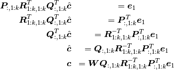
This procedure is very efficient and robust. The dominated computation cost
comes from QRCP, i.e. , where is some measure of the
size of local problems. It’s worth noting that QRCP is called only once
for each of the local problems.
| [1] | R. Conley, T. J. Delaney, and X. Jiao. Overcoming element quality dependence of finite elements with adaptive extended stencil FEM (AES-FEM). Int. J. Numer. Meth. Engrg., vol. 108, pp. 1054–1085, 2016. |
Improving the Strategy of Choosing Local Stencil
The original DTK2 stencil choice is based on a global configuration
parameter of either knn (k nearest neighborhoods) or radius. Moreover,
the resulting neighbors are used to be the support of the local problems, i.e.
number of points used in the Vandermonde systems. This procedure is not robust
for problems with point clouds that are not uniformly distributed. To overcome
this, we have implemented the following three steps for querying and choosing
local supports.
- Perform
knnsearch with a small number of neighborhoods to estimate the radii of the one-ring neighborhood of the local point clouds, say .
. - Perform
radiussearch with a relatively large radius so that we have enough candidates for next step. The radius is chosen as: .
. - Choose the support stencil, i.e. from the candidates
based on the number of columns (coefficients) in the Vandermonde systems,
i.e.
 . Notice that
 are 3, 6, and 10 for dimension (subscript
  ) 1, 2,
and 3 for quadratic polynomial basis functions, respectively.
) 1, 2,
and 3 for quadratic polynomial basis functions, respectively.
Note
We choose  for candidate selections and observe that better
results can be obtained with
for candidate selections and observe that better
results can be obtained with  .
.
Note
Theoretically, steps 1 and 2 can be achieved with knn search if we can
determine the number points in step 3. However, since we have ran into
robustness issues with DTK2 while using knn as the primary search
mechanism, we rely on the radius search.
With this strategy, the user doesn’t need to provide a radius. However, we still believe using topology based query is still efficient and better, but this requires meshes, which is an arduous task for this work.
Automate Parallel Mesh Rendezvous
While use DTK2 in parallel, each operator is built based on the cartesian bounding box the target point cloud with an approximated extension. For this extension length, we have implemented the following strategy:
(14)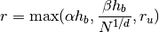
Where  is the longest edge in the cartesian bounding box,
  is the number of nodes, is the topological dimension, and
  is user-provided radius extension. Notice that the second term essentially
tries to estimate the average cell-size of the point cloud.
is user-provided radius extension. Notice that the second term essentially
tries to estimate the average cell-size of the point cloud.
Note
We choose  (10%) and
  as default
parameters.
as default
parameters.
Adaptation with Non-smooth Functions
A common challenge of solution/data remapping is to handle non-smooth
functions, i.e. avoiding Gibbs phenomenon.
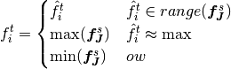
We apply a simple bounding strategy that enforces the transferred solutions
are bounded locally with respect to the sources values in the stencil
.
Given the intermediate solutions  after applying
the WLS fitting, then the following limitation is performed:
after applying
the WLS fitting, then the following limitation is performed:
(15)
In solution transfer, the strategy above may crop high-order values to first order in smooth regions, this is particularly true when the two grids resolutions differ too much from each other. Therefore, we need a mechanism that can pre-screen the non-smooth regions. We utilize a gradient based smoothness indicator, which is similar to those used in WENO schemes.
(16)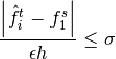
where
 .
This scheme is efficient and doesn’t require geometry data. The drawback is
also obvious—it’s too simple and tuning
.
This scheme is efficient and doesn’t require geometry data. The drawback is
also obvious—it’s too simple and tuning  is not easy.
Results
Convergence Tests
We have tested the AWLS on the following settings:
- plane surface,
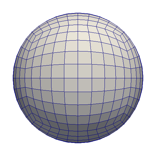
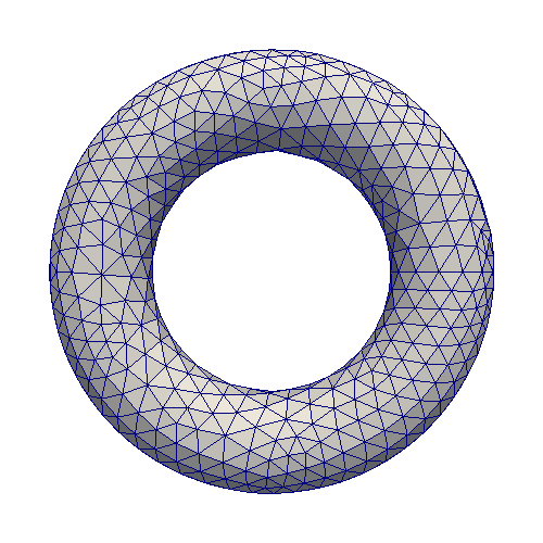
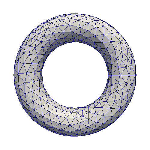
- spherical surface, and
- torus surface.
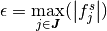
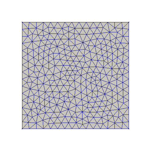
For the plane surface, we use structured grids on one side and triangular meshes on the other side. For setting 2, we use cubed-sphere grids and triangular meshes. For the last case, we use triangular meshes with different resolutions. All grids are uniformly refined by three levels in order to study the convergences. Notice that only the coarsest levels are shown in the following figures and all tests are transferred from fine grids to the corresponding coarse ones.
Finer Grids Coarser Grids 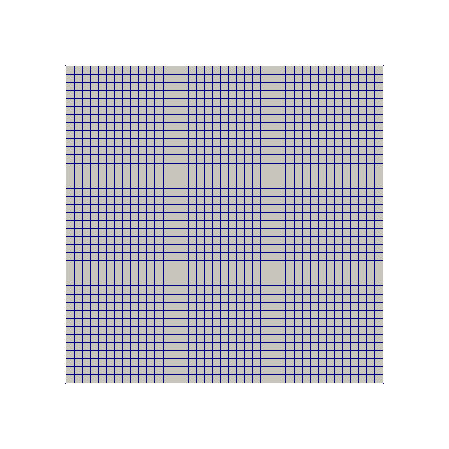
The convergence metric is:
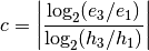
Where is some consistent measures of the grids. The error metric we
use is relative  errors:
For the plane surface, the following two models are tested:
 , and
, and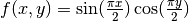 .
.
We use WENDLAND21 as weighting scheme and choose
 (18 points in stencils), the results are:
Convergence of the plane surface
For the 3D cases, we choose the following models:
 , and
, and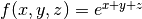 .
.
We use WENDLAND21 as weighting scheme and choose
 (32 points in stencils) for the spherical surface and
 (23 points in the stencils) for the torus surface, the results
are:
(23 points in the stencils) for the torus surface, the results
are:
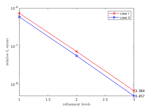
Convergence of the spherical surface
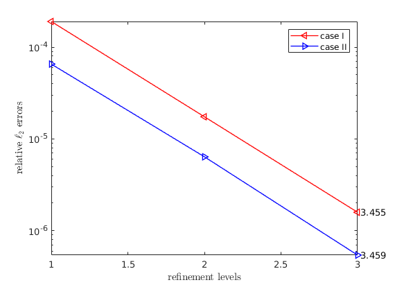
Convergence of the torus surface
Note that for all cases, the super-convergence phenomenon is observed, i.e.
the convergence rate is greater than  -st order.
The torus program script can be obtained here,
and the corresponding grids are stored in compressed npz file that can
be downloaded here.
Since the spherical surface is really special due to its smoothness and
symmetry, an almost- -nd order super-convergence can be obtained
with large stencils and
-nd order super-convergence can be obtained
with large stencils and WU2 weighting schemes. The
following results are with  (68 points in stencils):
However, this is less practical and hard to apply on general surfaces. As a matter of fact, we didn’t observe this with the torus setting.
You can obtain the test grids in VTK hear.
Non-smooth Functions
As a preliminary report, we perform the discontinuous test with the heaviside
function on the plane surface with  . The results are:
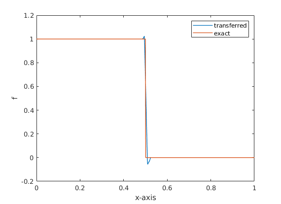
Heaviside function w/o resolving non-smooth regions
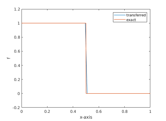
Heaviside function with resolving non-smooth regions
Usage
In order to use AWLS, you need to install the DTK2 package from my personal forked version.
Note
I didn’t decide to make a PR due to DTK2 is probably deprecated in the official repository???
To determine the backend DTK2, a static member function is implemented:
>>> from parpydtk2 import *
>>> assert not Mapper.is_dtk2_backend()
To enable AWLS support, you just need to call
awls_conf():
>>> mapper.awls_conf()
The default settings are:
methodis set toAWLS,basisis set toWENDLAND21, is set to 0.1 in (14),
 is set to 5 in (14),
 is set to 3 for
choosing local stencils
is set to 3 for
choosing local stencils
A complete list of parameters are:
>>> mapper.awls_conf(
...     ref_r_b=...,
...     ref_r_g=...,
...     dim=...,
...     alpha=...,
...     beta=...,
...     basis=...,
...     rho=...,
...     verbose=True,
... )
Where ref_r_b and ref_r_g are in (14) for blue and
green participants. dim is the topological dimension used in (14),
which is important if you need to transfer surface data (90% cases) in 3D space
in order to estimate the proper of mesh cell sizes.
In order to resolve discontinuous solutions, you need to pass in at least one
additional parameter resolve_disc to
transfer_data():
>>> bf_tag, gf_tag = 'foo', 'bar'
>>> mapper.transfer_data(bf_tag, gf_tag, direct=B2G, resolve_disc=True)
The default is in (16) is 2. To use another value, simply
do:
>>> mapper.transfer_data(...,resolve_disc=True, sigma=...)
Note
Resolving discontinuous solutions only works with
AWLS method under CHIAO45 backend.